Riccardo Loggini
Cubemap Generation With OpenCV
Table of Contents
Why Generating Cubemaps
This article will focus on transforming an equirectangular projection texture map
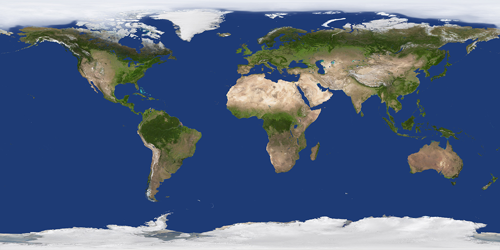
into a cube face texture
and eventually feed it into an application like NVidia Texture Exporter that can generate a cubemap DDS file with it.
I found myself in the need to texture both environment domes and spheres for my custom engine.
Cubemaps are de facto a standard format when wanting to texture an environment map in a graphics application. All the main graphics SDKs nowadays support cubemaps extensively.
They can also be used to texture any sphere object, such as a planet, like in the example of the previous chapter.
The problem, in general, is that most of the maps found online are in an equirectangular projection format, which “unwraps” the sphere texture into a 2:1 width-to-height size.
At that point, to generate a cubemap, we either have a software or tool that does it for us, or we need to build it ourselves.
When I decided to scan google for a “best” solution to my problems, I visited this StackOverflow thread where a user called Salix gave an exhaustive answer to the problem this blog post is explaining.
Still his solution is not the most performant and requires a C++ program to be run.
In the comments to his response, a user called Eric posted a python script which is using OpenCV to solve the same problem. This script is performing really well, and it uses a more professional approach to solve the problem.
At first, I did not fully understand the implementation, but liked the solution approach so much so that I’ve decided to make a post about it!
So there you go Eric, this is for you!
In pieces of software like commercial game engines, this process can be automatically handled, but I found it really useful to understand how these conversions work, and how to use a texture manipulation SDK as OpenCV in Python for this purpose.
It will now follow a series of trigonometric notions that will be needed to understand the implementation chapter.
They were made as much math beginner-friendly as possible, but basic notions of trigonometry from the reader are taken for granted.
Note: In all the formulas, domain of functions is not discussed (e.g. where the function does not exist or does not converge to a finite value) since for this article it has a secondary importance, but apologies in advance for that!
Polar Coordinates
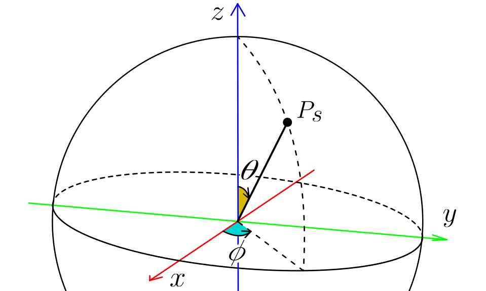
Each point on the sphere can be expressed by the polar coordinates mapping:
Where:
-
θ is the angle from the Z axis (inclination angle)
-
ɸ is the angle from the X axis on the XY plane.
Here follows a series of conversions between coordinates that will turn helpful later in the algorithm used to generate the cubemap.
From Polar To 3D Sphere
\[(x,y,z) \rightarrow(r \sin(\theta) \cos(\phi), r \sin(\theta) \sin(\phi), r \cos(\theta))\]The mapping follows:
All of them can be obtained with these trigonometric reason of the rect triangle:
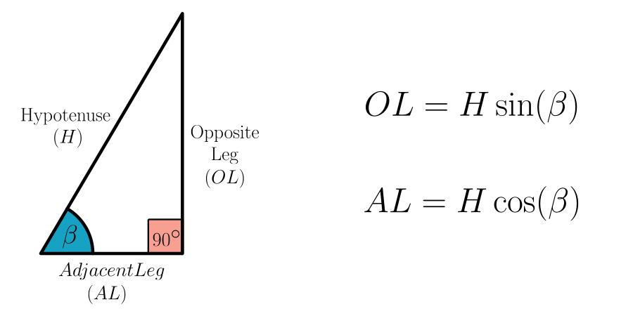
Starting from
\[z=r \cos(\theta)\]it’s because the adjacent leg (AL) of the rect triangle having radius r as the hypotenuse (H).
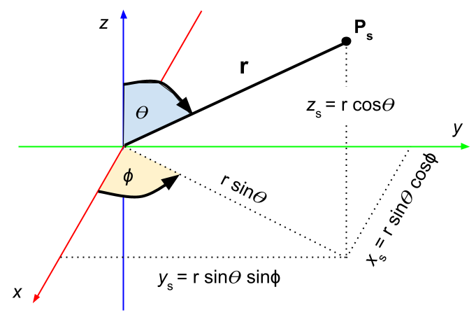
Speaking about the opposite leg (OL) which equals to r*sin, turns out that can be also seen as the hypotenuse of the rect triangle concerning the ɸ angle, and so we can repeat the same formula to deduce value of x and y.
-
$x=r \sin(\theta) \cos(\phi)$
-
$y=r \sin(\theta) \sin(\phi)$
Since x and y components are respectively the adjacent and opposite leg of the right triangle defined with angle ɸ and having hypotenuse size sin.
Cube Surrounding A Unit Sphere
Generating a cube map in this case has a lot to do with considering a cube surrounding a sphere with unit radius, in a way such that the cube also having x,y and z coordinates spanning in the interval [-1,1].
If we imagine the panorama image “wrapping” the sphere all around, what we want to do is to project every point of the wrapped image into the faces of the cube.
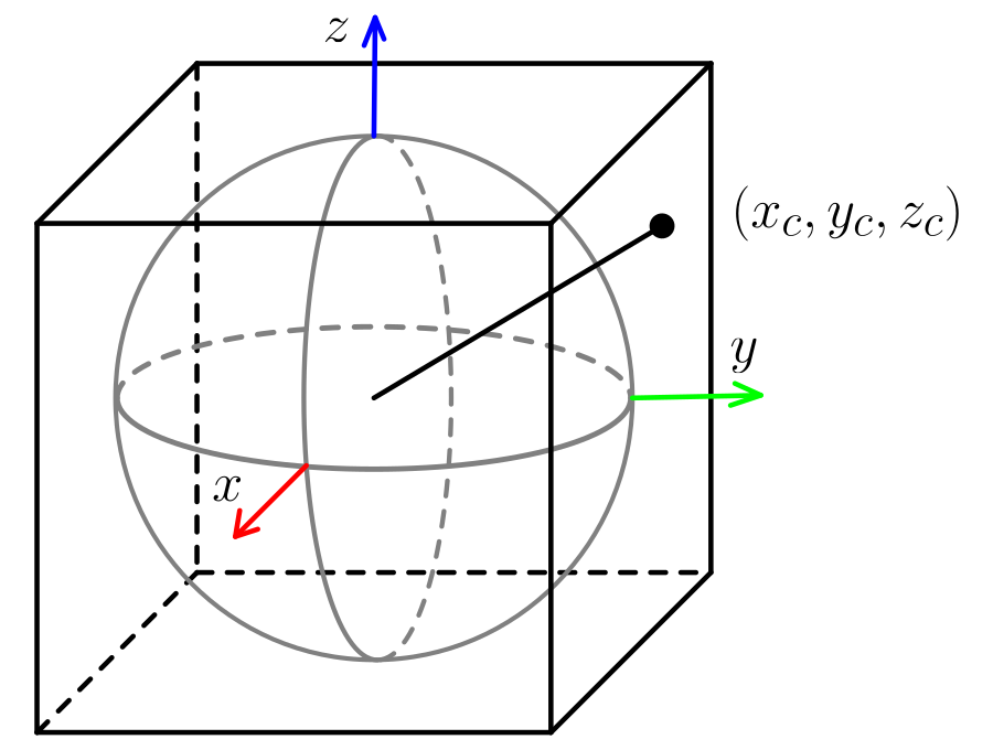
Of course this can be done in multiple ways, and here a specific solution among those is adopted.
The cubemap generation algorithm that will follow in the implementation, will start from texels of the cube face and it will need to retrieve the corresponding texel to sample in the panorama image.
To do that, it will need a function which, given a texel in the output cubemap image, will retrieve the corresponding polar coordinates on the sphere.
From Cubemap Image To Polar
Starting from a texel in the output cube face image, in order to retrieve the corresponding polar coordinates, an intermediate step is needed:
-
From Output Texel to 3D Cube Coordinates
-
From 3D Cube Coordinates To Polar
From Output Texel To 3D Cube Coordinates
Since we are starting with the output image, let’s first see what information we have at our disposal.
For each texel:
-
2D texel coordinates: here called $(x_f,y_f)$
-
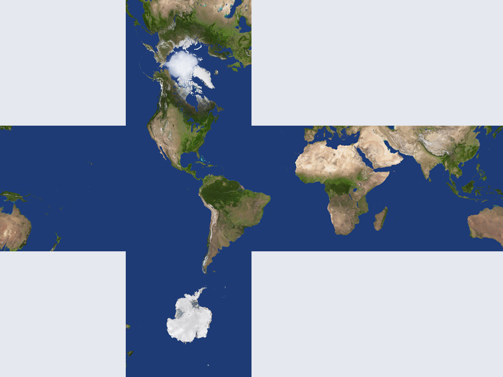
The face it belongs: this is up to the programmer to decide what layout to use and the order of the horizontal faces. The horizontal cross shape used below is because this format is common among the required for many software that generate cube map files. More on this at the end of the article.
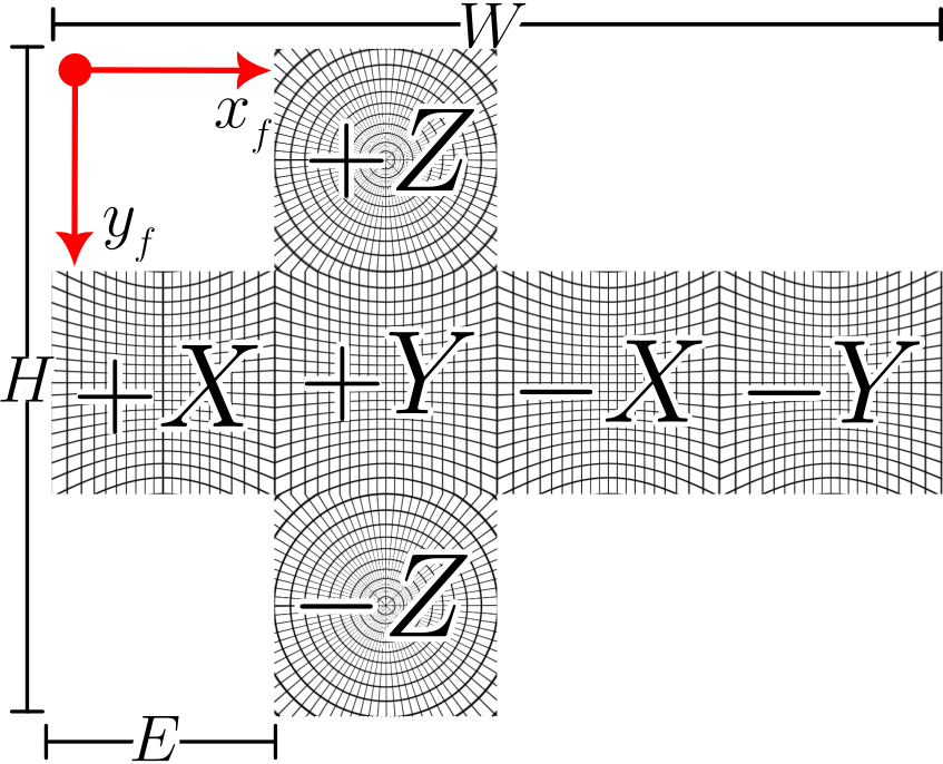
Transformation changes depending of course on the layout we use and which face we handle.
Be W and H the width and height of the output cube face image, and $E=W/4=H/3$ the edge size of a single cube face.
Given a pair $(x_f,y_f)$ and the face they are relative to, we can retrieve the $(x_c,y_c,z_c)$ coordinates on the 3D cube as:
- X-positive face
-
$x_c=1$
-
$y_c=-[1-2 \frac{x_f}{E}]=(2*x_f/E)-1$
-
$z_c=1-2 \frac{y_f-E}{E}=3-(2*y_f/E)$
-
-
Y-positive face
-
$x_c=1-2\frac{x_f-E}{E}=3+(2*x_f/E)$
-
$y_c=1$
-
$z_c=1-2\frac{y_f-E}{E}=3-(2*y_f/E)$
-
-
X-negative face
-
$x_c=-1$
-
$y_c=1-2\frac{x_f-2E}{E}=5-(2*x_f/E)$
-
$z_c=1-2\frac{y_f-E}{E}=3-(2*y_f/E)$
-
-
Y-negative face
-
$x_c=-[1-2\frac{x_f-3E}{E}]=(2*x_f/E)-7$
-
$y_c=-1$
-
$z_c=1-2\frac{y_f-E}{E}=3-(2*y_f/E)$
-
-
Z-positive face
-
$x_c=1-2\frac{x_f-E}{E}=3-(2*x_f/E)$
-
$y_c=-[1-2\frac{y_f}{E}]=(2*y_f/E)-1$
-
$z_c=1$
-
-
Z-negative face
-
$x_c=1-2\frac{x_f-E}{E}=3-(2*x_f/E)$
-
$y_c=1-2\frac{y_f-2E}{E}=5-(2*y_f/E)$
-
$z_c=-1$
-
Note: Each mapping formula above is heavily influenced by both the position of the face in the final image AND what face we are mapping into.
Changing the order of horizontal faces or sliding the position of the “arms of the cross” will also change the mapping!
Note: In some of those formulas signs are inverted, specifically in: $y_c$ of X-positive, $x_c$ of Y-positive, and $y_c$ of Z-positive.
A “visual” explanation to that can be found in the fact that, in we place ourselves in the centre of the sphere, by looking at one of those faces, to an increase of the $x_f$ or $y_f$ in the final image, the corresponding coordinate on the 3D cube decreases.
For example, with Z-positive, the minimum value of $y_f$ coordinate, $y_f=0$, corresponds to the maximum value in the coordinate $y_c=1$ on the cube, because of how the face is layered out in the final image.
From 3D To Polar
When we have all the 3D positions on the cube, finding polar coordinates becomes relative standard practice: even if those points are on the cube, they can still be considered “projected” versions of their counterpart in the inner unit sphere.
Here it does not matter if we consider the point on the sphere or its projected point on the cube: they will both return the same angles in respect to polar coordinates.
We can then use the formulas defined earlier in the Polar Coordinates section.
All the terms used here will refer to the drawing found in the same section.
What will change in those formulas, is the radius: for the unit sphere, radius is 1, but for the projected point on the cube, that’s a variable measure.
Be r the distance between the center of the sphere and the point on the cube $[x_c,y_c,z_c]$, we can first quickly calculate angle ɸ with:
since x and y are the sine and cosine of the right-triangle defined by them and ɸ, still obtained with these trigonometric reason of the rect triangle.
With the same triangle in mind, we can calculate the size of projection of r into the xy plane as:
\[r \sin\theta=\sqrt{(x_c)^2+(y_c)^2}\]as that can be seen as the hypotenuse of the same triangle, so it can be calculated with the Pythagorean theorem.
That term is needed since it can directly bring to find with:
\[\frac{z_c}{r \sin\theta} = \frac{r \cos\theta}{r \sin\theta} =\cot(\theta)\]Still in the algorithm implementation, this last step is transformed into:
\[\frac{r \sin\theta}{z_c}=\tan\theta\Rightarrow \theta = \arctan(\frac{r \sin\theta}{z_c})=\frac{\pi}{2}-\arctan(\frac{z_c}{r \sin\theta})\](by using trigonometric formulas) and this was done because we can make the same use of arctg function from the API.
Implementation
There are a multitude of ways and (pretty much all) languages we can use to build an image like we are doing in this article, like shown in this stack overflow thread.
I’ve decided to go for python because of the speed it can achieve and the easy setup.
Used Tools
This use case is implemented using
-
Windows 10
-
Powershell command window
-
Python 3.10.6
Regarding Python, the following modules are used:
-
numpy : Tools for scientific computation, used for its fast n-dimensional arrays.
-
sys : Access to system variables and functions from the interpreter (usually comes with Python)
-
PIL : Python Imaging Library, used for image file manipulation.
NumPy N-Dimesional Arrays
N-Dimesional array is a type of container that allows the manipulation of data at fast speed.
In python it’s identified by the shorter name ndarray.
Each object has single data type, a fixed size and can have multiple dimensions.
They also store the following properties:
-
shape : a tuple stating the length of each dimension.
-
dtype : the data type for the array.
The ndarray can be initialized in various ways. This implementation will make use of numpy.zeros:
my_array = numpy.zeros(<array shape>, dtype=<data type>)
for example
out_mapping = numpy.zeros((1024, 768, 2), dtype="f4")
will be an array containing floats, having 3 dimensions statically sized as 1024, 768 and 2.
The algorithm is also going to use the transpose of the ndarray, that can be accessed by ndarray.T, and allows to “split” the array into their dimensions:
dim1, dim2, dim3 = myarray.T
so to be able to use each dimension independently.
These arrays will be mainly useful for their parallel execution with multiple data of the same type: to generate an image we are dealing with texels, doing many operations of the same type, at the same time.
More info about ndarrays can be found at this scypy page.
Remapping Image with OpenCV
OpenCV will be used for only one but essential function call: cv2.remap
This function will find the texel values for the specified output mapped coordinates, by sampling an input image.
It takes the following input:
-
src: Input image, where to sample data from.
-
dst: Output image data, with the same data type as src, and matching size for map_x and map_y.
-
map_x: n-array of texel mapping for coordinate x.
-
map_y: n-array of texel mapping for coordinate y.
-
interpolation: The type of interpolation to use when sampling the input image. In this case, a cv2.INTER_LINEAR type will be used.
It returns the remapped array of texel data.
In our case, map_x and map_y we can use 2 numpy 3-dimensional arrays.
Their dimensions will be
-
[out_pixel_rows, out_pixel_colums, x_coord_mapping] -
[out_pixel_rows, out_pixel_colums, y_coord_mapping]
Be dst the output image, src the input image, the remap algorithm internally works as follows:
for each texel (x,y) in dst:
    get (x’, y’) coordinates from [map_x, map_y]
    sample src at (x’, y’)
    apply value to (x, y)
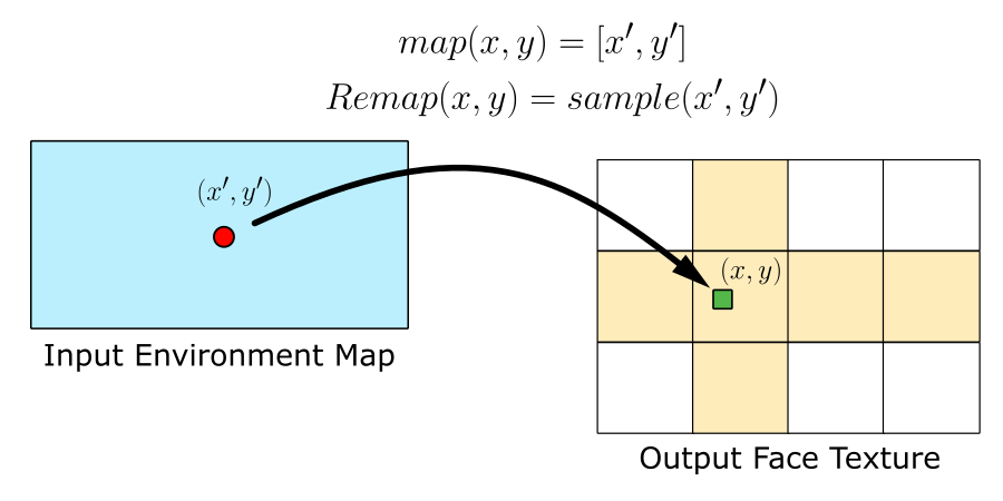
More about the remapping function can be found in the official documentation.
Store To Image File
To store the output texel array from the remapping function, the PIL library was used with Image.fromarray.
The following code will store the image fine in png format and open the file afterwards.
imgOut = Image.fromarray(cubemap_faces_data)

imgOut.save("output_faces.png")

imgOut.show()
Generate Mapping Data
All the main logic of this process is focused on generating mapping data (in form of texel x,y coordinates).
The focus is to reconstruct, for each texel of the output image, the xy-coordinates used to sample the input texture and retrieve the corresponding colour value.
The function starts by defining the output size: be E di edge of the output cube faces, the output needs to have a width of 4 times E, and a height of 3 times E, as this is the expected format to generate cubemaps (at least for the NVidia generator, more on this later).
def generate_mapping_data(image_width):
    # Output texture is 4 by 3 format (required by cubemap generators)
    out_tex_width = image_width
    out_tex_height = image_width * 3 // 4
    # Each cube face covers a quarter of the output image width
    face_edge_size = out_tex_width / 4

    # Create our numpy arrays
    out_mapping = numpy.zeros((out_tex_height, out_tex_width, 2), dtype="f4")
    xyz = numpy.zeros((out_tex_height * out_tex_width // 2, 3), dtype="f4")
    vals = numpy.zeros((out_tex_height * out_tex_width // 2, 3), dtype="i4")

    start, end = 0, 0
    # Here we are computing a "horizontal cross" made of cube map faces, since that's the format
    # most software need to generate a cubemap file.
    # This algorithm will go by pixel columns.
    # Interested pixels per column are mostly between face_edge_size and face_edge_size * 2
    # which will cover "the body" of the cross.
    # Apart from those, the pixels per column when rendering "the arms" of the cross, are going
    # to cover the whole column, and so from 0 to face_edge_size * 3.
    pix_column_range_1 = numpy.arange(0, face_edge_size * 3)
    pix_column_range_2 = numpy.arange(face_edge_size, face_edge_size * 2)
    # For each pixel column of the output texture ( so from 0 to width excluded)
    for col_idx in range(out_tex_width):

        face = int(col_idx / face_edge_size)
        # Each column will compute pixels in the "central strip" of the texture
        # Except for face 1 where we compute the "arms of the cross" which range
        # will interest every pixel of the column.
        col_pix_range = pix_column_range_1 if face == 1 else pix_column_range_2

        end += len(col_pix_range)
        vals[start:end, 0] = col_pix_range
        vals[start:end, 1] = col_idx
        vals[start:end, 2] = face
        start = end

    # Top/bottom are special conditions
    # Create references to values of each dimension of vals
    col_pix_range, col_idx, face = vals.T
    # Set each face index value where column pixel range less than cube face size, to 4.
    # That's because in the horizontal cross, face 4 it's the only face having this condition.
    face[col_pix_range < face_edge_size] = 4  # top
    # Equivalently, every face value where the column pixel range is greater or equal 2 times the
    # size of a cube face, belongs to face 5.
    face[col_pix_range >= 2 * face_edge_size] = 5  # bottom

    #-- Function continues.. --
From Texel To 3D Point On Cube
After having all the interested texel coordinates of the output image, and their relative face they belong to, the next step is to find their corresponding point on the 3D cube.
This is done with the process explained in section From Output Texel To 3D Cube Coordinates.
The n-dimensional arrays in this case allow to compute all the 3D points for a single face using one code line each, due to repeat the same operation for each tuple entry.
Aside from that, in the formulas defined earlier, the following terms appear in all the transformations:
-
$a=(2*x_f/E)$
-
$b=(2*y_f/E)$
so they can be used here in arrays to shorten the code syntax.
    # Convert from texel coordinates to 3D points on cube
    a = 2.0 * col_idx / face_edge_size
    b = 2.0 * col_pix_range / face_edge_size
    one_arr = numpy.ones(len(a))
    for k in range(6):
        # Here face_idx points to the values of vals where face equals to the current face index k
        face_idx = face == k

        # Create helper arrays with same dimension as face_idx
        one_arr_idx = one_arr[face_idx]
        a_idx = a[face_idx]
        b_idx = b[face_idx]

        if k == 0: # X-positive face mapping
           vals_to_use = [one_arr_idx, a_idx - 1.0, 3.0 - b_idx]
        elif k == 1: # Y-positive face mapping
           vals_to_use = [3.0-a_idx, one_arr_idx, 3.0 - b_idx]
        elif k == 2: # X-negative face mapping
           vals_to_use = [-one_arr_idx, 5.0 - a_idx, 3.0 - b_idx]
        elif k == 3: # Y-negative face mapping
           vals_to_use = [a_idx - 7.0, -one_arr_idx, 3.0 - b_idx]
        elif k == 4: # Z-positive face mapping
           vals_to_use = [3.0 - a_idx, b_idx - 1.0, one_arr_idx]
        elif k == 5: # bottom face mapping
           vals_to_use = [3.0 - a_idx, 5.0 - b_idx, -one_arr_idx]

        # Assign computed values for the dimesions of xyz pointed by face_idx
        xyz[face_idx] = numpy.array(vals_to_use).T

    #-- Function continues.. --
From 3D To Polar
The next step is to take those 3D points on the cube, and find their corresponding polar coordinates on the inner unit sphere.
The explanation for this step is found in the previous subchapter From 3D To Polar.
    # Convert to phi and theta
    x, y, z = xyz.T
    phi = numpy.arctan2(y, x)
    # Be r the vector from the sphere origin to the point on the cube
    # here r_proj_xy=r*sin(theta) and z=r*cos(theta), that's why below theta=pi/2 - arctg(z,r_proj_xy)
    r_proj_xy = numpy.sqrt(x**2 + y**2)
    theta = pi / 2 - numpy.arctan2(z, r_proj_xy)

    #-- Function continues.. --
Mapping Polar Coordinates to Input Texels
When we have polar coordinates corresponding to the points on the cube, the last step is to generate the mappings for x and y that point to locations in the input texture to sample.
    # From polar to input texel coordinates
    # Note: The input texture is assumed to be sized
    # width = 4.0 * face_edge_size
    # height = 2.0 * face_edge_size
    uf = 4.0 * face_edge_size * phi / (2.0 * pi) % out_tex_width
    vf = 2.0 * face_edge_size * theta / pi

    out_mapping[col_pix_range, col_idx, 0] = uf
    out_mapping[col_pix_range, col_idx, 1] = vf

    return out_mapping[:, :, 0], out_mapping[:, :, 1]
Wrapping All Up
The entire script can be downloaded clicking on this link:

Thanks again to Salix alba and Eric for the input in this Stack Overflow post.
From Cubemap Texture To DDS File
This section is for who needs to convert the just created output file into a DDS cubemap file ready to be handled by DirectX.
From all the methods I’ve found in the internet, the most reliable and updated was using the
NVidia Texture Tools Exporter.
They have 2 versions of that tool: a standalone and a Photoshop plugin.
The Photoshop plugin will ultimately open the standalone version of the tool when saving the current texture as DDS file, so that’s essentially the same process.
In the web page mentioned above there is also a video explaining how to use the plugin.
The tool expects a cubemap texture having a 3 by 4 aspect ratio (like the one we generated just before) or an OpenGL cubemap texture format that here we’ll not consider.
It should make available to select the Texture Type as Cube Map.
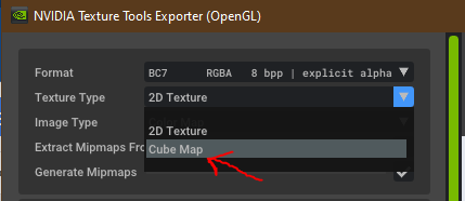
When done with the settings (format, mips, etc.) the last thep is pressing Save on the bottom right.
If all went well, the file should be ready to be used in a graphics application.
This ends the blog post. All started from an equirectangular projection map, all the way down to the corresponding cubemap dds file ready to be used in a graphics application.
With the hope this read was useful to you as for me it was to make it, wish you the best graphics programming and thanks for the read!
Sources
-
NVidia DDS Generator (PS Plugin)
https://developer.nvidia.com/nvidia-texture-tools-exporter -
Stack Overflow - Generating Cubemap Image
https://stackoverflow.com/questions/29678510/convert-21-equirectangular-panorama-to-cube-map Special thanks to Salix alba and Eric -
Jason Brownlee - Introduction to NumPy Arrays in Python
https://machinelearningmastery.com/gentle-introduction-n-dimensional-arrays-python-numpy/ -
Research Gate - Yoandry Rivero’s Trigonometry Board
https://www.researchgate.net/figure/Trigonometry-Formula_fig3_328777687 -
OpenCV Remap Function Question
https://stackoverflow.com/questions/46520123/how-do-i-use-opencvs-remap-function -
Python Pillow Module
https://pillow.readthedocs.io/en/stable/reference/Image.html -
Earth Texture - Solar System Scope
https://www.solarsystemscope.com/textures/