Riccardo Loggini
From HLSL To CUDA
Table of Contents
Why CUDA In Graphics
GPUs already had an important role in general purpose computing before AI, in scientific and engineering simulation, cryptography and data processing, to name a few, but the spread of generative models has pushed GPU engineering skills into much higher demand.
Applications are changing as fast as the hardware, and as a GPU specialist I feel it’s important to keep up with what the market is asking for.
I’m writing this post as an introduction to CUDA from a graphics software engineer perspective.
The following content can be seen as a continuation read from my previous post about compute shaders.
CUDA is an NVIDIA API for GPGPU: General-Purpose computing on Graphics Processing Units.
It refers to using a GPU’s massively parallel architecture for computation beyond the traditional rasterization pipeline.
If this sounds familiar, yes, it’s the same Single Instruction, Multiple Threads (SIMT) execution model behind every compute shader you’ve written in D3D12.
CUDA is NVIDIA’s own C++-based platform for this, predating and running in parallel to standardized compute shader APIs.
In the mid-2000s, before compute shaders existed, people did GPGPU by disguising computation as a rendering pass, writing results to a render target via a full-screen pixel shader, then reading it back (e.g. Fast matrix multiplies using graphics hardware).
CUDA (2007) and later compute shaders in D3D11/Vulkan gave GPGPU workloads a proper first-class entry point, with no rendering-pipeline disguise required.
A few concrete places GPGPU work, often CUDA specifically, shows up in modern real-time and offline graphics pipelines:
- Ray tracing. NVIDIA’s OptiX framework (CUDA-based) powers GPU-accelerated ray tracing and, notably, the denoisers used in production renderers like Arnold. Denoising a noisy path-traced image is exactly the kind of general-purpose parallel workload CUDA was built for.
- Physics and simulation. Cloth, fluid, and particle simulations (NVIDIA Flex and GPU PhysX) use GPGPU compute to parallelize what would otherwise be sequential per-particle or per-constraint updates.
- Sorting and stream compaction. GPU-driven pipelines lean heavily on primitives like radix sort and stream compaction — for visibility culling, transparency sorting, indirect draw generation. CUDA’s Thrust library provides mature, heavily-optimized implementations of these that are harder to hand-roll efficiently in a compute shader.
- Offline tooling. Lightmap baking, texture synthesis, and other asset-pipeline tasks that run outside the real-time frame budget are common candidates for CUDA, since portability across GPU vendors isn’t a constraint for a build-time tool the way it is for a shipping game. The Unity Progressive Lightmapper, for example, uses OpenCL for its core path-traced bake, and it offers optional NVIDIA Optix denoiser.
- AI-driven image reconstruction. Deep-Learning Super Sampling (DLSS) and similar upscaling/frame-generation techniques run neural network inference on Tensor Cores accessed through NVIDIA’s proprietary NGX SDK. This is arguably the most consequential use of GPGPU in graphics right now, as it changed the performance budget for an entire generation of renderers. (How this squares with the interop cost described below is worth a closer look. See the note under “Tight integration with the frame”).
CUDA Or Compute Shader?
As listed before, a number of graphics applications use CUDA in their computation workflow, then when and why should I still use a compute shader?
Where compute shaders win
Tight integration with the frame. A compute shader dispatch lives on the same command list, uses the same resource-binding and barrier infrastructure, and slots into a render graph exactly like any other pass. CUDA/D3D12 interop is possible, but it means bridging two separate runtimes with explicit shared-resource handles and fence-based cross-API synchronization (an overhead you don’t want to pay for something like a per-frame post-process pass). Example: GPU-driven occlusion culling generating indirect draw arguments that feed directly into the next draw call on the same queue. A CUDA kernel here would need to hand results back across an API boundary before the GPU could even issue the draw.
Isn’t DLSS a counterexample? It runs every frame and it’s CUDA/Tensor-Core work, so it looks like it should pay the interop cost just described, but it doesn’t, and that’s not an accident. DLSS isn’t invoked as a raw CUDA kernel with a context switch; it goes through NVIDIA’s NGX SDK, whose
NVSDK_NGX_D3D12_EvaluateFeaturecall takes your application’s own D3D12 command list as an argument and records the Tensor Core inference inline, the same way any other pass would be. There’s no separate CUDA context, no shared-resource handle, no fence-based sync visible to the engine. That inline path is a privilege of NVIDIA’s own driver stack, not something available to third-party CUDA code. NVIDIA built NGX this way precisely because the interop cost is real, and DLSS wouldn’t be shippable at real-time rates without sidestepping it.
No cross-context latency. Anything that has to happen every frame, in lockstep with the rest of the pipeline, is cheaper and simpler as a compute shader than as a CUDA kernel with an interop round-trip. Examples include tile-based light culling, particle simulation updates and TAA resolve.
Cross-vendor portability. CUDA is for NVIDIA-only hardware. Anything shipping on AMD, Intel, or console hardware (PS5 and Xbox are both AMD GPUs) simply cannot depend on it (more on the alternatives in the next chapter).
Where CUDA wins
Library ecosystem. CUDA nowadays offers very mature and hand-tuded libraries which leverage the underlying hardware at maximum capacity, covering linear algebra, FFTs, deep learning primitives, and multi-GPU communication. To name a few: cuBLAS, cuDNN, cuFFT, Thrust, CUTLASS, TensorRT, NCCL. Example: training or running inference for a DLSS-style upscaling network needs cuDNN/TensorRT-class primitives — there’s no compute-shader equivalent with comparable performance.
Profiling depth. Nsight Compute gives per-kernel occupancy, register pressure, warp execution efficiency, and memory-throughput breakdowns — a level of introspection RenderDoc or PIX don’t match for compute shader dispatches. When you actually need to know why a kernel is slow, this matters.
A richer language. CUDA is C++ which brings templates, classes, recursion, dynamic parallelism (kernels launching kernels), unified memory. HLSL is a much more constrained with C-like shading language up to ShaderModel 5.1 and some C++ from HLSL2021.
Genuinely real-time, without NGX-style special-casing. As stated before, DLSS avoids the interop cost by never crossing an API boundary at all, but there’s a separate category of application that wins with CUDA at real-time or interactive rates for the opposite reason: there’s no D3D12/Vulkan frame graph to bridge into in the first place, because the whole render loop is CUDA-native from the start. Examples: interactive viewport renderers in DCC tools (Blender Cycles X, NVIDIA Omniverse’s RTX Renderer, Redshift, Chaos Vantage), and video/stream AI effects that sit outside a game’s frame graph entirely, like NVIDIA Broadcast or RTX Video Super Resolution.
Limitations And Alternatives
CUDA’s limitations
The core limitation, as anticipated before, is that CUDA only runs on NVIDIA GPUs. Code written against it cannot run on AMD, Intel, or mobile GPUs without a translation layer or a rewrite.
On top of that, there are factors including cost, architecture fragmentation and sub-optimal Api architecture decisions.
- Architecture fragmentation. Compute capability differs across GPU generations (
sm_75,sm_86,sm_89,sm_90, …), so shipping code either targets specific architectures at compile time or falls back to PTX JIT-compilation at runtime (a versioning concern a fixed-ISA target like a CPU doesn’t have). - Low-level responsibility. Manual memory management, explicit shared-memory tiling, and hand-tuning occupancy/register pressure are all on you: this is the same trade-off as HLSL vs. a higher-level engine abstraction, just one level lower. (More on how Triton addresses this below.)
- Cost and availability. part of the price tag on NVIDIA’s data-center GPUs isn’t there because the silicon itself is worth that much more than a competitor’s chip. It’s there because CUDA’s ecosystem lock-in lets NVIDIA charge more than pure hardware competition would allow, and people still pay it rather than deal with the cost of switching to something cheaper. Cloud GPU capacity on NVIDIA hardware is also routinely supply-constrained.
OpenCL
OpenCL is the original cross-vendor answer to CUDA: running across GPUs, CPUs, and even Field-Programmable Gate Arrays (FPGAs) and Digital Signal Processors (DSPs). OpenCL 3.1 shipped in 2026 with mandatory SPIR-V ingestion, and layered implementations now run OpenCL over Vulkan and D3D12, widening availability even to platforms without a native driver.
- Pros: genuinely vendor-neutral: open standard with public conformance testing, can target the widest range of hardware of anything in this list.
- Cons: NVIDIA treats OpenCL as a compliance checkbox rather than a first-class target. It ships a conformant driver but doesn’t invest in it the way it does CUDA, so performance on NVIDIA hardware specifically tends to lag. OpenCL’s actual center of gravity today has shifted toward mobile and embedded (Arm, Imagination, Qualcomm), not data-center GPU compute. There’s no equivalent to cuBLAS/cuDNN-level library maturity, and the API itself is considerably more verbose and lower-level than CUDA’s runtime API. Explicit platform/device/context/queue setup for even a simple kernel launch. In practice, most people today reach OpenCL indirectly, through a higher-level layer like SYCL, rather than writing it by hand.
HIP / ROCm (AMD)
HIP (Heterogeneous-Compute Interface for Portability) and ROCm (Radeon Open Compute). AMD’s answer, deliberately designed to look like CUDA: the HIPify tool auto-converts large amounts of existing CUDA source, and hipcc can even compile HIP to run on NVIDIA hardware by wrapping CUDA underneath, giving a degree of two-way portability.
- Pros: the lowest-friction migration path if you already have CUDA code and want AMD hardware support; open source.
- Cons: ROCm’s tooling and library ecosystem is younger and less battle-tested than CUDA’s, with a history of rougher Windows support (improving, but real). And because HIP mirrors CUDA so closely, it doesn’t raise the abstraction level at all. You’re still responsible for the same manual tiling and memory management, just retargeted.
SYCL
SYCL is Khronos’ modern single-source C++ model for heterogeneous compute (implemented via Intel’s oneAPI/DPC++, AdaptiveCpp, and others), able to target CPUs and GPUs from multiple vendors by compiling down to CUDA, HIP, Level Zero, or OpenCL depending on backend.
- Pros: standard, modern C++ — templates, lambdas, no special language extensions the way CUDA/HLSL need. Genuinely portable across hardware vendors from a single source tree.
- Cons: the ecosystem and tooling are still maturing relative to CUDA’s. Performance portability is alwats tricky to achieve. Getting genuinely competitive performance across every backend from one source remains a real, generally unsolved problem, not just a marketing claim.
Triton
Triton is where GPU-compute hiring in the job market is actually heading right now. Triton is a Python-embedded language (@triton.jit-decorated functions) where you reason about block-level tiles rather than individual threads. The compiler automatically handles memory coalescing, shared-memory allocation, and thread scheduling underneath. It compiles through an MLIR-based pipeline down to PTX for NVIDIA or AMDGCN for AMD.
- Pros: dramatically less code than hand-written CUDA for common kernel shapes (matmul, fused elementwise ops, attention), while still getting PTX that competes with hand-tuned CUDA. FlashAttention, for example, ships an official Triton reference implementation alongside its hand-tuned CUDA kernel. It’s the default kernel-generation backend for PyTorch 2.x’s
torch.compile, and vLLM’s attention backends (PagedAttention, RoPE, RMSNorm) are written in it. AMD support has matured quickly too (ROCm 6.2+, covering both CDNA data-center and increasingly RDNA consumer GPUs). Even NVIDIA is investing in it directly — a CUDA Tile IR backend for Triton, targeting Blackwell’s tensor cores, was announced in early 2026. - Cons: minimum NVIDIA compute capability is 8.0 (Ampere and newer — Volta/Turing, e.g. V100/T4, aren’t supported). You’ll need to give up the fine-grained control needed to hand-optimize the last few percent of performance, and it’s tuned primarily for the access patterns common in ML kernels (block-structured matmul, reductions, fused elementwise ops) rather than arbitrary general-purpose kernels a graphics engineer might reach for. It’s also conceptually still Python/ML-ecosystem-shaped, not a general systems language the way CUDA C++ or HIP are.
What’s best then
If you’re specifically aiming at the ML/AI-infra job direction discussed earlier in this series, Triton is arguably more relevant to learn alongside CUDA than as a replacement for it. It’s rapidly becoming the productivity layer the industry writes kernels in day to day, with raw CUDA reserved for the cases where Triton’s abstraction doesn’t fit.
If cross-vendor portability is the hard requirement, HIP is the least-friction path if you’re starting from CUDA, otherwise SYCL if you want to start clean in modern C++.
Terminology
Two terms show up constantly and are worth pinning down first.
The host is the CPU and its process: your regular C++ program, doing memory allocation, file I/O, and launching kernels, the same role your D3D12 application code plays.
The device is the GPU itself: the thing every kernel actually executes on, and what every cudaMalloc/cudaMemcpy call allocates on or moves data to and from.
Code and qualifiers are either host-side (__host__, the implicit default for a plain function) or device-side (__global__, __device__), and the CUDA Runtime API is the bridge between the two, the same way a command queue is the bridge between your D3D12 app and the GPU executing its command lists.
A kernel is a C++ function marked __global__ that runs on the GPU. It’s the direct equivalent of an HLSL compute shader’s entry point, the function carrying the [numthreads(x,y,z)] attribute.
Launching a kernel means invoking it from host (CPU) code with the kernel<<<gridDim, blockDim>>>(args) syntax. This doesn’t run the function once: it tells the GPU how many blocks (gridDim) and how many threads per block (blockDim) to spawn to execute that same function body in parallel, one invocation per thread, equivalent scheduling a Dispatch(x, y, z) call performs for a compute shader’s numthreads-sized thread groups.
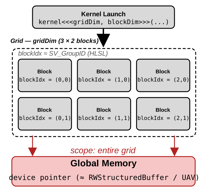
A kernel launch spawns a grid of blocks — the same dispatch/group nesting a compute shader has, just with CUDA’s own names for each level. Buffers passed in as plain device pointers are global memory, visible to every block and every thread in the grid, the same way a RWStructuredBuffer is visible to an entire dispatch.
Then inspecting a single block:
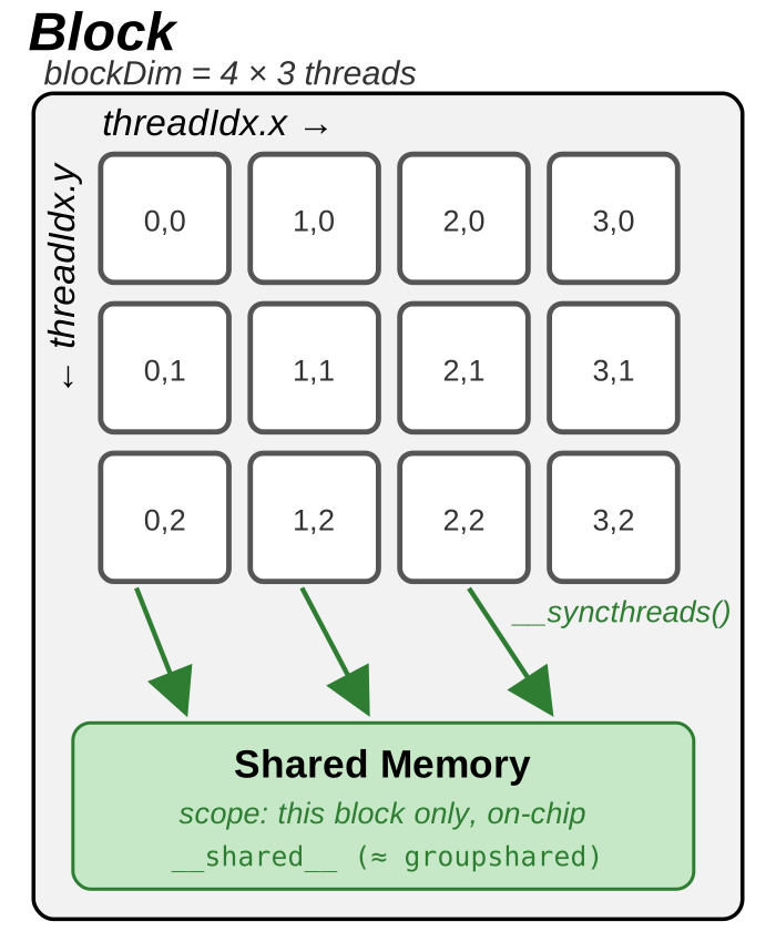
Each block is itself a group of threads, indexed by threadIdx the way SV_GroupThreadID indexes a thread within a group. groupshared memory maps to __shared__: allocated per block, visible only to the threads inside that block, and fast because it’s on-chip. Its state is synchronized with __syncthreads(), CUDA’s equivalent of GroupMemoryBarrierWithGroupSync().
| HLSL / D3D12 compute | CUDA equivalent |
|---|---|
Dispatch(x, y, z) |
kernel<<<gridDim, blockDim>>>(...) |
numthreads(x,y,z) attribute |
blockDim (set at launch, not in the kernel) |
SV_GroupID |
blockIdx |
SV_GroupThreadID |
threadIdx |
SV_DispatchThreadID |
computed manually: blockIdx * blockDim + threadIdx |
groupshared |
__shared__ |
GroupMemoryBarrierWithGroupSync() |
__syncthreads() |
| RWStructuredBuffer / UAV via root signature/descriptors | plain device pointer, passed as a kernel argument (CUDA’s binding model is much simpler with no descriptor tables) |
dxc (HLSL compiler) |
nvcc |
| PIX / RenderDoc | Nsight Systems (timeline) / Nsight Compute (per-kernel profiling) |
Wave intrinsics (WaveActiveSum, 32-lane on NVIDIA hardware) |
warp-level primitives (__shfl_sync, cooperative groups) — same 32-thread warp under the hood, since it’s the same silicon |
Hardware
A modern GPU packs thousands of simple cores designed for high-throughput, data-parallel work, backed by memory bandwidth far exceeding a CPU’s. Understanding where a kernel’s blocks and threads actually land in silicon, and what memory they land near, explains most of the “why is my kernel slow” questions Nsight Compute exists to answer.
Compute Hierarchy: GPC → SM → Warp
A CUDA-capable chip is partitioned into GPCs (Graphics Processing Clusters), each containing several Streaming Multiprocessors (SMs).
The SM is the real unit of scheduling: when a kernel launches, the hardware scheduler assigns each block from the grid to exactly one SM, where it stays resident for its entire lifetime, sharing that SM’s resources with however many other blocks fit alongside it.
Each SM packs:
- CUDA cores: the scalar FP32/INT32 ALUs that execute the bulk of ordinary kernel code.
- Tensor Cores: fixed-function matrix multiply-accumulate units, the hardware DLSS’s NGX SDK drives underneath (see the AI-driven image reconstruction bullet earlier).
- Warp schedulers: issue instructions to warps, groups of 32 threads that execute in lockstep on the SM’s ALUs.
blockDimthreads get sliced into warps of 32 under the hood regardless of how you shapednumthreads/blockDim: this is the actual SIMT execution granularity, one level below the logical thread/block model from the Terminology section above. - Register file and L1/shared memory: the fast, on-chip storage partitioned among the warps and blocks resident on that SM (more below).
- Special Function Units (SFUs) and load/store units: transcendental math (
sin,rsqrt, …) and memory-access plumbing, respectively.
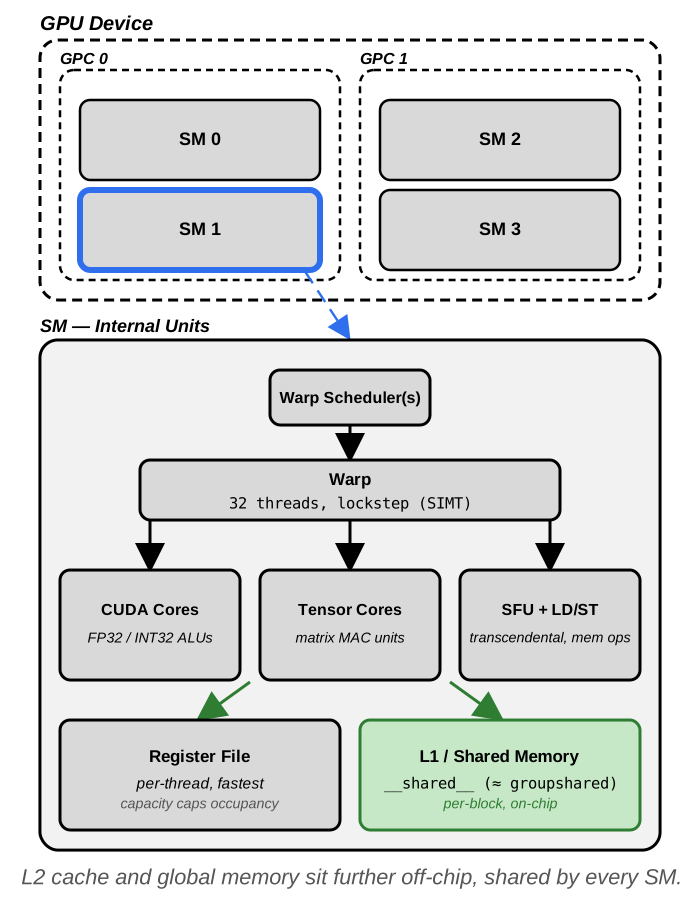
Because a block is pinned to one SM, blockDim doesn’t just describe your problem’s shape: it directly determines how many warps a block occupies, and therefore how many blocks can fit on an SM at once. Threads within a warp that take different branches (an if some threads enter and others skip) don’t run in parallel: the warp serializes both paths and masks off the inactive threads, the closest CUDA equivalent to a compute shader’s wave/subgroup divergence cost.
For example, NVIDIA RTX 5090 architecture has 11 GPCs holding 170 SMs in total, each SM packing 128 CUDA cores and 4 Tensor Cores (21,760 CUDA cores and 680 Tensor Cores across the whole chip), with 4 warp schedulers per SM keeping up to 48 resident warps, 1,536 threads, in flight at once. Each SM also carries a 64K-entry (256 KB) register file and up to 128 KB of L1/shared memory: the exact pool blockDim and __shared__ allocations are drawn from, and the numbers occupancy calculations divide against. (source)
Memory Hierarchy
Every level of the compute hierarchy above has a matching memory tier, and the tiers get larger and slower the further they sit from the ALUs:
| Tier | Scope | Relative speed |
|---|---|---|
| Registers | per-thread | fastest, smallest |
| Shared memory / L1 | per-block, lives on the owning SM | fast, on-chip — this is __shared__ / groupshared |
| L2 cache | chip-wide, shared by every SM | slower than L1, still on-chip |
| Global memory (DRAM) | entire grid, every kernel | slowest, largest and the off-chip GDDR/HBM behind every plain device pointer |
GDDR and HBM are the two DRAM types GPUs use for that off-chip pool:
GDDR (e.g. GDDR6X, GDDR7): what consumer/gaming cards use, including the RTX 5090’s 32 GB of GDDR7. Discrete chips around the GPU package on the board, connected over a wide bus (512-bit on the 5090).
HBM (e.g. HBM2e, HBM3): what datacenter GPUs use (A100, H100, MI300, …). Instead of separate chips on the board, several DRAM dies are stacked vertically and placed right next to the GPU die on a shared silicon interposer — much wider bus, much higher bandwidth per pin, but more expensive to manufacture, which is part of why it’s reserved for datacenter parts.
Two more special-purpose paths worth knowing: constant memory, a small cached region for read-only values broadcast to every thread (the closest CUDA relative of a constant/uniform buffer), and texture memory, which routes reads through the GPU’s dedicated texture units — the same fixed-function hardware a pixel shader’s Sample() call hits, still reachable from a kernel via a cudaTextureObject_t when its 2D-locality caching or built-in filtering is useful. local memory is the odd one out: despite the name, it isn’t a separate fast tier, it’s register-spill data that actually lives in global memory — which is why register pressure (too many live values for the register file) quietly costs you global-memory bandwidth.
That same RTX 5090 backs its 170 SMs with 98 MB of L2 cache shared chip-wide, sitting in front of 32 GB of GDDR7 global memory delivering 1,792 GB/s over a 512-bit bus. Constant memory doesn’t scale with the chip the way L2 and global memory do: it’s a fixed CUDA architectural limit, 64 KB total, cached through an 8 KB working set per SM, on this card just as on any other. (source)
Getting On And Off The Chip
The GPU is still a peripheral: it’s attached to the host system over PCIe, or over NVIDIA’s own higher-bandwidth NVLink for GPU-to-GPU and, on some systems, GPU-to-CPU links. Still, these connections matters in specific setups only, like doing multi-GPU work with NCCL.
Dedicated copy/DMA engines move data across that link independently of the SMs, which is what makes cudaMemcpyAsync genuinely asynchronous: a kernel can keep computing on last frame’s data while this frame’s input is still in flight, the same overlap a D3D12 copy queue running alongside a direct queue gives you.
Not every specialized unit on the die is reachable from plain CUDA C++ at all: RT Cores (BVH traversal and ray-triangle intersection, exposed through OptiX) and the Optical Flow Accelerator (motion-vector generation behind DLSS Frame Generation) sit next to the SMs and are driven through their own NVIDIA SDKs rather than a __global__ kernel.
How This Shapes Performance
Nsight Compute’s per-kernel metrics all trace back to the hardware above:
- Occupancy: how many warps are resident on an SM at once, capped by whichever resource runs out first: registers, shared memory allocated per block, or the SM’s max warp/block count. Low occupancy means the scheduler has fewer warps to switch between when one stalls. A warp “stalls” when the next instruction it needs to issue can’t execute yet, so the warp scheduler sets it aside and can’t make progress on it that cycle. The scheduler then looks for a different resident warp that is ready to issue, and runs that one instead.
- Latency hiding: a GPU has no CPU-style branch predictor or deep out-of-order window. It hides memory latency by parking a stalled warp and issuing another resident one instead. This is why occupancy matters: too few resident warps and the SM idles waiting on DRAM instead of hiding that wait behind other work.
- Memory coalescing: when the 32 threads of a warp touch contiguous global-memory addresses, the memory controller merges them into a handful of wide transactions, scattered per-thread addresses fragment into many small ones. Bandwidth utilization drops accordingly.
- Shared-memory bank conflicts: shared memory is physically split into 32 banks. When multiple threads in a warp hit the same bank in the same instruction, those accesses serialize instead of completing in one cycle.
- Tensor Core utilization: hitting peak throughput needs the right data types and tile shapes (FP16/BF16/TF32/INT8, dimensions aligned to the core’s native tile size). Code that doesn’t match falls back to CUDA cores and leaves most of the SM’s matrix-multiply throughput unused.
Example Usage
To see the terminology and hardware model above land in actual code, cuda-cubemap is a small CUDA port of the equirectangular-to-cubemap conversion from Cubemap Generation With OpenCV: same algorithm (map each output cube-face texel to a 3D direction, convert that direction to spherical coordinates, bilinearly sample the input panorama at the resulting longitude/latitude), moved from Python/NumPy/OpenCV to a __global__ CUDA kernel running one thread per output pixel.
Before diving into code, here’s the shape of the whole program: what runs on the host, what runs on the device, and where the two boundaries (the H2D/D2H copies from the Nsight Systems section below) actually sit.
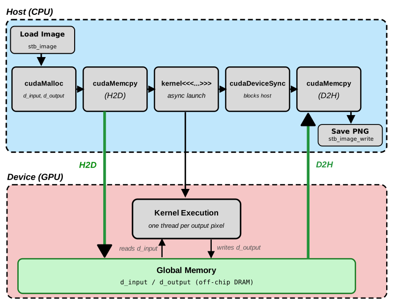
The kernel launch itself is asynchronous: cudaLaunchKernel returns to the host immediately, which is why cudaDeviceSynchronize further down the host lane is a separate, explicit blocking call rather than something implied by the launch. On the device side, every thread reads from d_input and writes to d_output independently, both living in global memory, the same off-chip pool discussed in the Memory Hierarchy section, with no __shared__ traffic between threads at all.
The Kernel
The kernel signature and dispatch index come directly from the Terminology table above:
__global__ void equirectToCubemapCrossKernel(
    const unsigned char* __restrict__ input, int inputWidth, int inputHeight,
    unsigned char* __restrict__ output, int outputWidth, int faceSize)
{
    int x = blockIdx.x * blockDim.x + threadIdx.x;
    int y = blockIdx.y * blockDim.y + threadIdx.y;

    if (x >= outputWidth || y >= 3 * faceSize)
        return;

    // ...face/direction/spherical-coordinate math, then a bilinear sample...
}
__global__ is the qualifier that makes this a kernel: a function that runs on the device but is callable from host code, exactly the [numthreads(x,y,z)]-attributed entry point of a compute shader.
blockIdx.x * blockDim.x + threadIdx.x is the SV_DispatchThreadID row from that table, written out by hand since CUDA doesn’t compute it for you.
__restrict__ is CUDA’s spelling of C99/C++’s pointer-aliasing hint: it tells nvcc that input and output never overlap, which is what allows more aggressive load/store scheduling.
The bilinear sample itself lives in a separate function marked __device__ instead of __global__:
__device__ void sampleBilinear(const unsigned char* img, int width, int height,
                                float u, float v, unsigned char* outPixel)
__device__ is the third CUDA-specific function qualifier (alongside __global__ and host-only, unmarked functions): it can only be called from other device code, never from the host, which C++ alone has no concept of, there’s no equivalent access restriction on a plain function.
Launching the kernel is where the kernel<<<gridDim, blockDim>>>(...) syntax from the Terminology section shows up for real:
dim3 blockDim(16, 16);
dim3 gridDim((outputWidth + blockDim.x - 1) / blockDim.x,
             (outputHeight + blockDim.y - 1) / blockDim.y);

equirectToCubemapCrossKernel<<<gridDim, blockDim>>>(
    d_input, inputWidth, inputHeight, d_output, outputWidth, faceSize);
dim3 is CUDA’s built-in 3-component vector type for launch dimensions, the gridDim/blockDim equivalent of a numthreads-shaped Dispatch(x, y, z) call.
The ceiling-division for gridDim is the same pattern a compute shader dispatch needs whenever the image size isn’t an exact multiple of the thread-group size, so a partially-filled group at the border reads/writes out of bounds unless the kernel itself checks (that’s what the if (x >= outputWidth || ...) return; guard above is for).
Picking a 16 × 16 block also isn’t arbitrary: that’s 256 threads, exactly 8 full warps, so no lane in any warp goes idle from a badly-shaped block.
Host Side: Getting Data To And From The GPU
The host driver in main.cu is where the “CUDA’s binding model is much simpler” shows up. No descriptor heaps, no root signature, no resource-state transitions: just a handful of C-style Runtime API calls moving flat device pointers around.
CUDA_CHECK(cudaMalloc(&d_input, inputBytes));
CUDA_CHECK(cudaMemcpy(d_input, h_input, inputBytes, cudaMemcpyHostToDevice));

launchEquirectToCubemapCross(d_input, inputWidth, inputHeight, d_output, faceSize);
CUDA_CHECK(cudaDeviceSynchronize());

CUDA_CHECK(cudaMemcpy(h_output.data(), d_output, outputBytes, cudaMemcpyDeviceToHost));
cudaMalloc/cudaMemcpy/cudaFree are the global-memory allocate/upload/download calls behind every plain device pointer discussed in the Memory Hierarchy section.
cudaDeviceSynchronize() is the host-side wait for the kernel to finish: since input, kernel and output all live in the same CUDA context, there’s no fence-based cross-API synchronization.
More on the specific syntax can be found in the CUDA official guide.
Where The Performance Comes From
The original Python/OpenCV version processes the whole output image through vectorized NumPy array operations and a single cv2.remap call: fast for CPU code, but still bound to a handful of CPU cores (plus SIMD width) and paying Python/NumPy per-call dispatch overhead between each vectorized step.
The CUDA port instead launches one thread per output pixel, tens of millions of them for a large cross image, and every thread’s work (pick a face, build a direction vector, convert to spherical coordinates, bilinearly sample) is entirely independent of every other thread’s.
There’s no __shared__ memory and no __syncthreads() anywhere in this kernel: with zero data reuse between neighboring output pixels, there’s nothing to stage in on-chip memory, so the kernel is free to just spread across as many resident warps as the GPU can schedule and let latency hiding do the rest.
The math itself, atan2f, sqrtf, floorf, fminf/fmaxf, is exactly the transcendental workload the SFUs from the Compute Hierarchy section, while the bilinear sample’s four texel fetches and lerp belong to the load/store units.
Debug And Profile CUDA
NVIDIA’s Nsight suite is the CUDA-native counterpart to PIX/RenderDoc, split across a few purpose-built tools rather than one single application:
- Nsight Systems: a system-wide timeline correlating CPU calls, kernel launches, memory copies and their overlap across streams, the first stop for “where is the time actually going” questions (covered below).
- Nsight Compute: a per-kernel deep dive, occupancy, register pressure, warp execution efficiency, memory-throughput breakdowns, for once the slow kernel is already found and the question becomes why (also covered below).
- Nsight Visual Studio Edition: integrates a CUDA-aware debugger directly into Visual Studio, breakpoints and stepping through device code, register/local-memory watch windows, the same workflow as debugging host C++ code.
cuda-gdbis the command-line equivalent on Linux. compute-sanitizer(the successor to the now-deprecatedcuda-memcheck): a correctness-checking suite catching out-of-bounds/misaligned global-memory accesses, shared-memory race conditions, uninitialized reads, and incorrect__syncthreads()usage, CUDA’s equivalent of ASan for device code.
cuda-gdb, compute-sanitizer, and both Nsight profilers ship with the CUDA Toolkit installer; Nsight Systems and Nsight Compute are also available as standalone downloads (updated on their own, faster cadence), and Nsight Visual Studio Edition has its own installer.
Nsight Systems (timeline)
Hardware used for this capture. The profile below was captured on an NVIDIA GeForce RTX 4080, the machine cuda-cubemap actually ran on, not the RTX 5090 used for the spec numbers in the Hardware section above. The two aren’t meant to line up: the 5090 figures are architecture reference points, this capture just reflects whatever GPU happened to be in the dev machine.
Nsight systems documentation can be found at this link.
Worth defining:
- H2D = Host-to-Device (uploading data from CPU/system RAM to the GPU, e.g.
cudaMemcpyHostToDevice) - D2H = Device-to-Host (downloading results from the GPU back to CPU/system RAM, e.g.
cudaMemcpyDeviceToHost).
Capturing a profile of cuda-cubemap from the Example Usage section above shows the shape you’d expect from a program that does one image, once: a single stream, no overlap, with the GPU timeline laid out as three back-to-back blocks, an H2D cudaMemcpy, the kernel, and a D2H cudaMemcpy. Nothing runs concurrently: no cudaMemcpyAsync, no second stream, so each phase blocks the next.
Capturing this profile. cuda-cubemap has a VS Code task for this: Tasks: Run Task > “nsys: profile and open report” builds the project, profiles it against the sample texture, and opens the resulting timeline directly in the Nsight Systems GUI, no manual
nsys profileinvocation needed. See the “Profiling with Nsight Systems” section of the repo’s README for the setup details (including the admin-privileges note for CPU context-switch/sampling data).
Nsight Systems’ process tree gives a cleaner, GPU-only version of that same story, scoped to actual device time rather than CPU API duration:
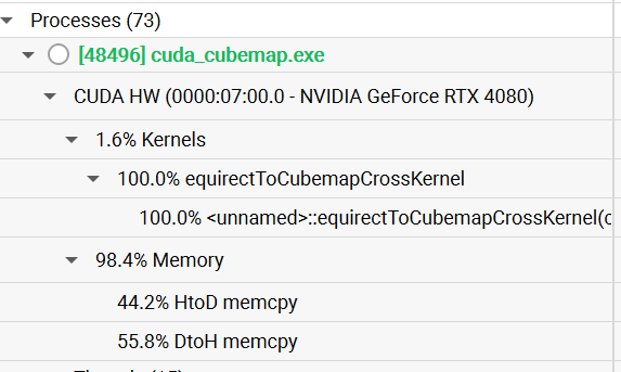
Kernels account for just 1.6% of GPU time against 98.4% for memory operations, the same “compute is cheap, transfer dominates” story detailed below, but without cudaMalloc’s context-init cost muddying it. It also splits the transfer itself: 55.8% DtoH against 44.2% HtoD, the download costing more than the upload, because the output horizontal-cross image ends up larger than the input equirectangular panorama.
The CUDA API Summary view is more interesting than the timeline shape alone:
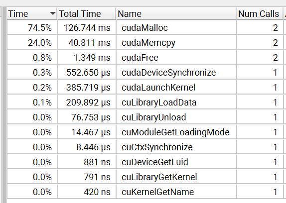
cudaMalloc dominates at 74.5% of total CPU-side API time (126.744 ms across 2 calls), but that’s not the cost of allocating device memory: it’s the CUDA runtime’s lazy context initialization (driver init, primary context creation, device enumeration) getting billed to whichever CUDA call happens to run first in the process. It’s a one-time cost, not a per-call one, the CUDA equivalent of a first-frame shader-compile stutter in D3D12: run this on a batch of images instead of one, and it’s paid once, not once per image.
cudaMemcpy (24.0%, 40.811 ms for the H2D + D2H pair) is the real cost worth discussing. The host-side image buffers here (stb_image’s output, a plain heap allocation) are regular pageable memory rather than pinned memory (cudaMallocHost/cudaHostAlloc), so the driver needs to stage every transfer through an internal pinned bounce buffer first.
Pinned memory (a.k.a. “page-locked” memory) is memory the OS has been told to lock in place at the fixed physical address, so it can never be moved or paged out.
Pageable memory can’t be transferred asynchronously at all.
The reason this distinction matters for cudaMemcpy specifically: the GPU’s DMA engine (mentioned in “Getting On And Off The Chip”) transfers data by reading/writing physical addresses directly, with no CPU involvement mid-transfer. That only works if the source/destination address is guaranteed stable for the whole transfer. Pageable memory gives no such guarantee, the OS could move that page while the transfer is in flight, so the driver can’t DMA from it directly. Instead, it first does a CPU-side copy from your pageable buffer into an internal pinned staging buffer, then DMAs from that staging buffer to the GPU, an extra copy you’re paying for on every cudaMemcpy.
With pinned memory, that staging step disappears: the DMA engine can transfer straight from your buffer, which is faster, and it’s also a hard requirement for cudaMemcpyAsync to actually be asynchronous, since an async transfer running in the background needs a source address guaranteed not to move while the CPU carries on.
The trade-off is that pinned memory is pageable memory taken away from the OS’s swappable pool, so it’s not something you’d want to use indiscriminately for every allocation, just for buffers that are actually transferred to/from the GPU repeatedly. That’s exactly the gap the cuda-cubemap example leaves on the table: its host buffers are plain pageable memory, which is part of why the cudaMemcpy numbers in the profile came out as high as they did.
Everything else in the table, cudaFree, cudaDeviceSynchronize, cudaLaunchKernel, module loading (cuLibraryLoadData and friends), adds up to under 1.5 ms combined: launch and module-loading machinery isn’t where the time goes.
The previous listed table image is CPU-side API duration, though, not GPU execution time. For that, the CUDA GPU Kernel Summary view is the right one:
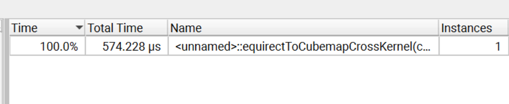
equirectToCubemapCrossKernel actually ran in 574.228 µs on the GPU, closely matching the 552.650 µs cudaDeviceSynchronize reported in the API table above (unsurprising, since blocking on the kernel’s completion is exactly what that call does). Set against the 40.811 ms cudaMemcpy total, the kernel is roughly 71× faster than the round trip that feeds it.
What the profile adds is the honest complication that “free compute” doesn’t mean “free end-to-end”: for a one-shot, run-once texture-pipeline tool like this one, a 41ms transfer cost is a non-issue, but the same ratio in a pipeline processing many images or frames back-to-back would make the transfer, not the kernel, the thing worth optimizing first.
Nsight Compute
Back at the start of this post, “Profiling depth” was listed as a place CUDA wins: Nsight Compute gives per-kernel occupancy, register pressure, warp execution efficiency and memory-throughput breakdowns. Here’s what those actually look like for equirectToCubemapCrossKernel, captured (with --set full, since the default set skips several of the sections below) on the same RTX 4080 as the Nsight Systems capture above.
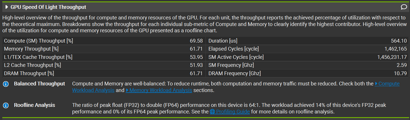
GPU Speed Of Light Throughput is the headline chart: Compute (SM) Throughput sits at 69.58%, Memory Throughput at 61.71%, and Nsight Compute’s own callout labels this “Balanced Throughput”, both need to come down to meaningfully speed up the kernel, neither is idle while the other maxes out. The roofline breakdown adds a specific detail worth checking: the kernel hits only 14% of this device’s FP32 peak (and, expectedly, 0% of FP64, nothing here uses doubles), despite that 69.58% overall SM throughput number. The gap between those two is the SFU pipe: atan2f, sqrtf and friends aren’t running on the FP32 FMA units the roofline percentage tracks, they’re running on the transcendental math hardware described in Compute Hierarchy, so a kernel can drive the SM hard without driving the FP32 pipe specifically. The reported duration, 564.10 µs, also lines up closely with the 574.228 µs from the Nsight Systems kernel summary, close enough to be normal run-to-run variance rather than a discrepancy worth chasing.
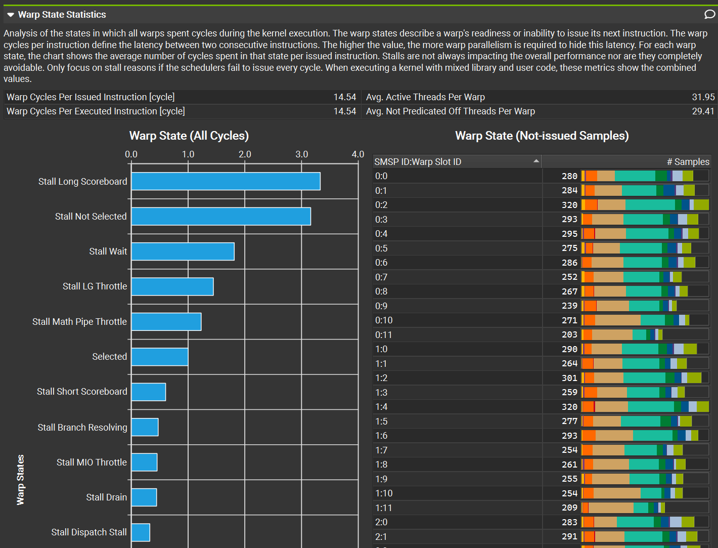
Warp State Statistics
Stall Long Scoreboard, a warp waiting on a global-memory load it issued, is the single largest bar: exactly the bilinear sample’s texel fetches fromd_input, each thread in a warp reading a different, data-dependent address because of the spherical-coordinate remapping, so those loads don’t coalesce as cleanly as a straight image copy would and the warp pays for it in latency.Stall Not Selectedis a close second, but that one isn’t a problem: it means a warp was ready to issue and the scheduler picked a different ready warp instead, a sign there’s enough parallelism resident to keep the SM fed, not a bottleneck.Stall Waitis next: a fixed-latency dependency stall, waiting on the result of a previous ALU/SFU instruction with known, constant latency, as opposed to a variable-latency memory load. The face → direction → spherical-coordinate math is a long chain of dependent scalar float ops (dx/dy/dzfeed oneatan2f, that feedsxyLen, that feeds a secondatan2f, and so on), each one waiting out the previous instruction’s pipeline latency before it can issue. It’s the cost of that dependency chain, unrelated to memory.Stall LG Throttle(Local/Global) is the load/store unit’s instruction queue being full: the warp can’t even issue its next memory instruction yet, separate fromLong Scoreboardwaiting on data already in flight.sampleBilinearissues four texel loads (p00/p10/p01/p11) per channel, timeskChannels = 3, up to twelve global loads per thread for one bilinear sample, enough LG traffic to back up the queue on its own.Stall Math Pipe Throttleshows up too, smaller but present, confirming the SFU-pressure point from the roofline chart above.
Divergence, by contrast, isn’t a factor here: Avg. Active Threads Per Warp is 31.95 out of 32, so the per-face branch and the boundary-check if barely cost anything.
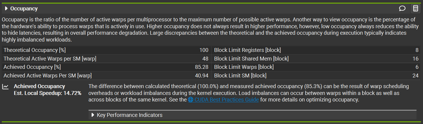
Occupancy closes the loop on a choice made back in “The Kernel”: the 16 × 16 (256-thread, 8-warp) block size.
Of the four block limits Nsight Compute reports, registers allow 8 resident blocks/SM and shared memory allows 16 (unsurprising, this kernel uses none), but the warp count is what actually binds: 48 max warps/SM ÷ 8 warps/block = 6 blocks/SM, which is exactly the reported Block Limit Warps.
That’s Theoretical Occupancy of 100%, no headroom left on the table by the block shape itself. Achieved Occupancy comes in at 85.28% (40.94 of 48 warps/SM), and Nsight Compute attributes that gap to scheduling overhead and workload imbalance rather than a sizing mistake, likely the tail end of the dispatch, where blocks covering the image’s last rows finish and drain at slightly different times.
It estimates a 14.72% local speedup if that gap closed, real, but not the kind of number that would change the conclusion from the Example Usage section: for a one-shot conversion tool, d_input’s coalescing and this occupancy gap are the two places left to optimize, and neither is worth chasing until this kernel runs inside something that calls it often enough for 564 µs to start adding up.
Sources
- CUDA from Wikipedia
- NVIDIA CUDA
- Fast matrix multiplies using graphics hardware
- NVIDIA OptiX
- Arnold Renderer
- NVIDIA Flex
- NVIDIA PhysX SDK
- CUDA Thrust
- Unity Progressive Lightmapper documentation
- OpenCL
- NVIDIA DLSS
- NVIDIA NGX Programming Guide
- NVIDIA Omniverse
- Working out CUDA Just-In-Time (JIT) compilation - vitalitylearning
- HIP documentation (AMD ROCm)
- ROCm (AMD)
- SYCL
- Triton
- MLIR
- NVIDIA Blackwell Tuning Guide
- NVIDIA GeForce RTX 5090
- Nsight Compute
- CUDA Programming Guide
- NVIDIA Nsight Developer Tools overview
- CUDA Toolkit downloads
- Nsight Systems downloads
- Nsight Visual Studio Edition